Problem1 - d
Examine the numerical errors for different schemes as a function of the grid spacing and the integration time step. Evaluate the spatial and temporal accuracy of the numerical schemes.
Here, temporal and spatial accuracies were evaluated using following parameter:
\[P_{temporal} = \frac{log(\frac{\phi_{2t} - \phi_{4t}}{\phi_{t} - \phi_{2t}})}{log(2)}\]
\[P_{spatial} = \frac{log(\frac{\phi_{2h} - \phi_{4h}}{\phi_{h} - \phi_{2h}})}{log(2)}\]
Euler equation (Pure convection problem)
In this test, the Euler-Explicit scheme was not employed because it is unconditionally unstable method for pure convection problem.
- Errors as a function of time step, dt
- The evaluation of time step change effect was done for single case of grid size, N = 4001.
- Crank-Nicolson scheme gives better accuracy over the entire set of test cases than Euler implicit, because the CR scheme is a second order accuracy in both space and time.
- In general the error drops monotonically with decrease of time step.
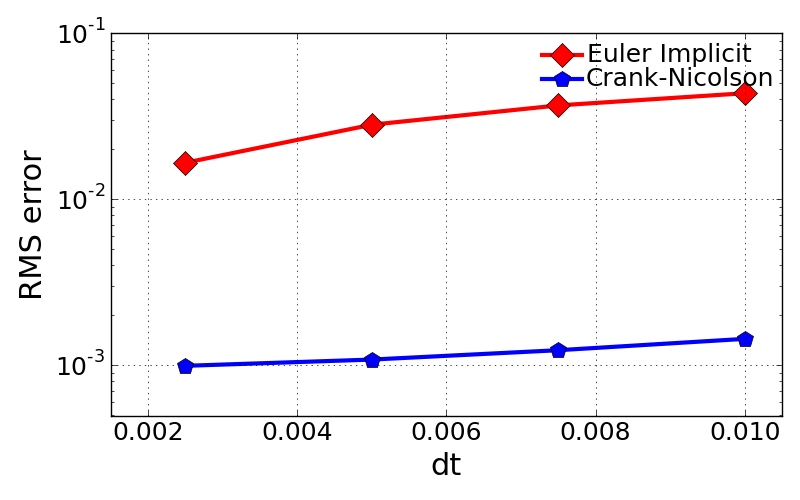
Courant no. (dt) EI CR 0.25 (0.0025) 0.0166148385052 0.00099101659914 0.5 (0.005) 0.0281716938047 0.00108091830901 0.75 (0.0075) 0.0368227088826 0.0012308579817 0.1 (0.01) 0.0436049875194 0.00144069783592
- Evaluation of temporal accuracy \(P_{temporal}\) defined below with different methods:
- \(P_{temporal}\) for EI = 0.4173
- \(P_{temporal}\) for CR = 2.0007
- Errors as a function of grid spacing
- The evaluation of grid resolution effect on error was done for single set of time step, dt = 0.005, so different Courant number.
- Increase of grid point number drops the error. But change of error is not much clear with Euler implicit.
- Flat profile of errors in Euler implicit case may suggest to run the simulation with much smaller number of grid points in order to see increasing errors with less grid points.
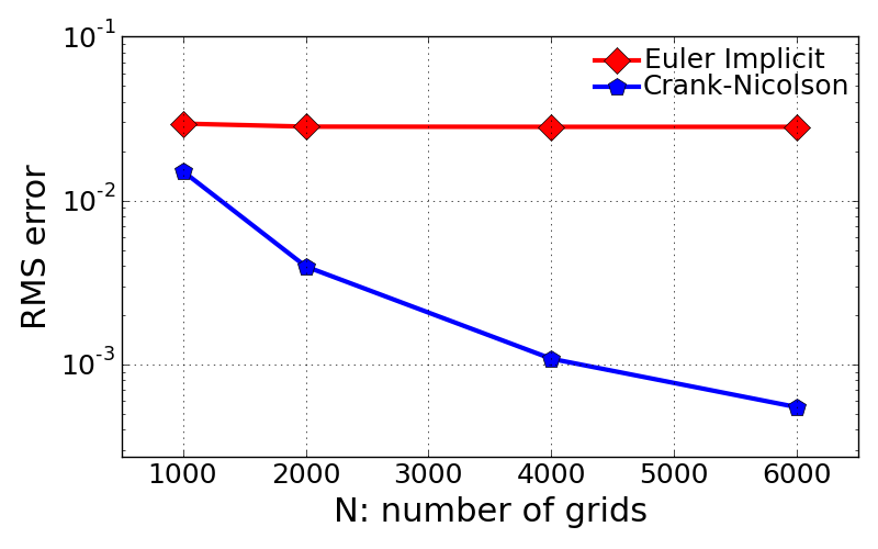
Number of nodes (Cr) dx EI CR 1001 (0.125) 0.04 0.0294768440151 0.0150567999236 2001 (0.25) 0.02 0.0282487385682 0.00395484817586 4001 (0.5) 0.01 0.0281716938047 0.00108091830901 6001 (0.75) 0.00667 0.0281685389275 0.000547240822165
- Evaluation of spatial accuracy \(P_{spatial}\) defined below with different methods:
- \(P_{spatial}\) for EI = 3.9946
- \(P_{spatial}\) for CR = 1.9497
Burger’s equation (Convection + Diffusion)
In this test, only a part of Euler-Explicit cases was employed for analysis because the method was unstable beyond certain value of Courant number.
- Errors as a function of time step, dt
- The evaluation of time step change effect was done for single case of grid size, N = 4001.
- As confirmed above, Crank-Nicolson scheme is much accurate compared to other two methods.
- Euler explicit and Euler implicit are showing very comparable error values each other, almost same order of magnitude.
- Getting error values over dt = 0.005 was not possible for Euler explicit.
- This suggest that Euler explicit should be run with Courant number less than 0.5.
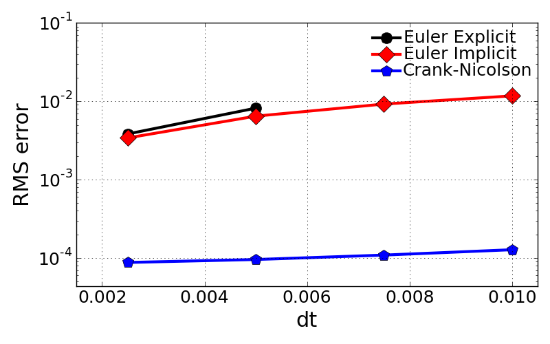
Courant no. (dt) EE EI CR 0.25 (0.0025) 0.00383043947008 0.00340998441819 8.76084904269e-05 0.5 (0.005) 0.00818535015496 0.00646574830074 9.55709046347e-05 0.75 (0.0075) inf 0.00922821563363 0.000108841001593 0.1 (0.01) inf 0.0117416771678 0.000127423869135
- Evaluation of temporal accuracy \(P_{temporal}\) defined below with different methods:
- \(P_{temporal}\) for EI = 0.7879
- \(P_{temporal}\) for CR = 2.0001
- Errors as a function of grid spacing
- Crank-Nicolson scheme shows dramatic change of RMS error value with different grid size as confirmed in Euler equation problem.
- Euler explicit and Euler implicit have same order of magnitude for their accuracy. This is because these two methods have same order of accuracy in both time and space.
- N = 6001 case was failed to get stable solution.
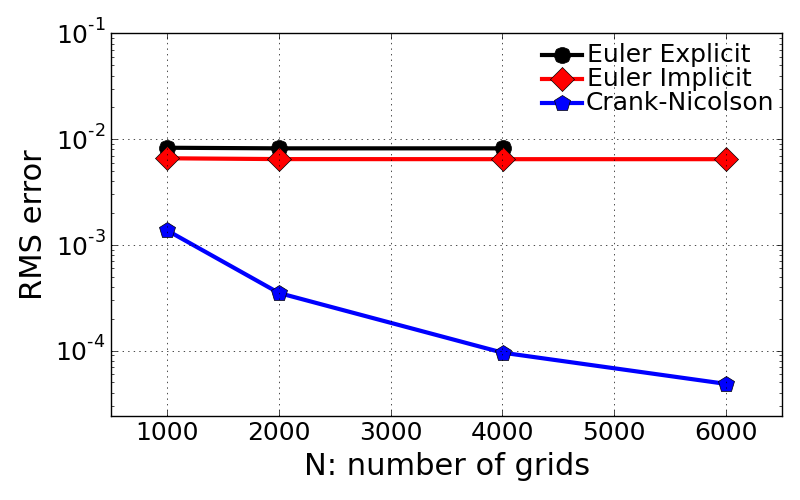
Number of nodes (Cr) dx EE EI CR 1001 (0.125) 0.04 0.00829334418324 0.00659287238512 0.00136897946621 2001 (0.25) 0.02 0.00818432743363 0.00647642954911 0.000350398456828 4001 (0.5) 0.01 0.00818535015496 0.00646574830074 9.55709046347e-05 6001 (0.75) 0.00667 inf 0.00646469348398 4.83756513792e-05
- Evaluation of spatial accuracy \(P_{spatial}\) defined below with different methods:
- \(P_{spatial}\) for EI = 3.4465
- \(P_{spatial}\) for CR = 1.9990